Can Computers Understand Our Emotions?
Facial Expression Recognition with PyTorch and Deep Learning using different Image Classification Techniques.

To answer the above question, we need to understand how computers actually see and build intuitions about what they see. But computers can’t see! Since they don’t have actual eyes, but there are tools and methods to help computers “see” things like humans can. The central component of all computer vision is images (with videos you work with a bunch of images). Computers see images as millions of individual pixels each with color and alpha values. There are lots of libraries and tools with which we can make computers see, some of the most popular ones are OpenCV, TensorFlow, PyTorch, MatLab, SimpleCV, SciPy, and NumPy.
In this blog, I will try to build a Deep Learning Image Classification Model which will be able to recognise the facial expression of human faces.
Approach:-
- Finding the dataset.
- Preparation/Cleaning/Pre-Processing of the dataset.
- Experimenting with different models.
- Comparing all the model's training time and accuracy.
- Finalizing our model for deployment.
Disclaimer: If you are too lazy to read all through the blogs, I have prepared a short and clear conclusion of whatever I have done in this whole process you can directly jump to the Conclusion section of this blog to get a rough idea about all of my approaches and their boundaries.
1. Finding/Exploring the dataset:
Since some of the datasets were too large and some of them were not that easy to work with for any beginner in DL Field, it took me almost one day to find this dataset. It contains 3 columns emotions , pixelsand Usage and 35,887 rows.Where emotions columns contained labels from 0–7as anger, disgust, fear, happiness, neutral, sadness, and surpriserespectively. But I found two minor problems i.e., the images in the pixelscolumns were in a string format and the whole dataset was in .csvformat and was not that easy to work for any beginner, so I created my own dataset from it.
2. Preparation of the dataset:
First of all, we need to import some of the libraries required to convert a string of pixels to an image of a .png format.
- Imports
- The
oslibrary will help us in creating directories for our different class images, and also it will help us to move through directories and create or delete directories. pandasandnumpylibraries help us in working with the different file formats and performing certain mathematical operations.PILlibrary helps us in working with images in Python.cv2is a library which can give vision to computer i.e., it helps us to work with the device camera.
2.1 Defining a function to convert any pixels of string to image.png
- Function Definition:
So, with the help of the above function, we just need to provide the label of the image i.e., 0–1 and it will convert all the pixels to an image matching with the condition provided inside the function. If you would like to have a look at the entire source code, You can find it here -> convert-pixels-to-images-in-one-go
We have completed our 10% task towards our final goal.
3. Experimenting with Image classification models and Techniques:
We will be experimenting with 4 different kinds of model:
- Logistic Regression Approach
- Feed-Forward Neural Network(FNN)
- Convolutional Neural Network(CNN)
- Convolutional NN with Data Augmentation & Regularization Technique
3.1 Logistic Regression Approach for Image Classification
Logistic regression is used to calculate the probability of a binary event occurring, and to deal with issues of classification. There are three different kinds of Logistic regression: Binary logistic regression, Multinomial logistic regression, and Ordinal logistic regression. In our case, we’ll be using Multinomial logistic regression. So, let’s start by importing the required libraries and packages.
Imports:
So, now let’s understand the dataset directory and file structures.
But before moving towards our codes, do make sure that you click on the New Notebook option of the dataset page i.e., here. In this way, we don't have to download the dataset. Also, we are working on Kaggle Kernels too.
Our dataset contains two dir and one file , with 7 classes as [‘anger’, ‘fear’, ‘surprise’, ‘happiness’, ‘sadness’, ‘neutral’, ‘disgust’].
Can we know the number of images in each class? Yes.
We can see that class happiness contains the highest number of images and class disgust the lowest.
Creating the dataset variable and converting each image to Tensors:
Now, after converting each image to Tensors, let’s have a look at a single image.
The first line of output signifies that our image is of 48*48 pixels and contains 3 channels i.e., RGB. But since our images are B/W, I didn’t think of converting them to channel 1 because in some cases images with 3 channels tend to work better with certain models.
But how are we going to visualize the images, will it not be a problem to view images in Tensors? So let's visualize them with the help of plt.imshow Finallyfunction from matplotlib library.
Function to plot the pixels or Tensors:
One thing to note from the above code is .permute(1,2,0) since the channel of the images is at first position but plt.imshow() requires the channel to be at the last position. so we use the .permute() function to do the required changes.
Now it’s time to view an image:
Preparing the training and test dataset:
We have allotted 10% of the dataset for the validation set. The dataset also contains an extra test set which we have allotted as test_ds.
Data Loaders: Data loaders help us in loading our dataset into batches, it also shuffles the sets each time we load the data into the model. Else if we would not use data loaders we will end up having only the happiness class or the sad class in a particular batch of data.
Let us also have a look at a batch of data:
So, now we have done all our tasks which are required before building any model.
Building the Model
Since we have built our model, we will require an accuracy function to check the accuracy while training the model, an evaluatefunction to evaluate our model each time we do some changes to find out which combination of hyperperParams gives the best result and also a fit function is required to do training task, with the capability of changing the no. of epoch andlr.
Defining the accuracy , evaluateand the fit function.
So far, we have defined our model and defined some of the useful functions which will be required to increase our performance of the model. So let’s have a look before the training how our model performs with the help of the evaluate function which we just defined.
We can see that without any training our model gives an accuracy of about 13% and with a very huge validation loss.
We are now ready to start the training of the model. At first, we keep the epoch as 45 and the lr as 0.01 so that our model understands how the tensors and tries varying the weight and biases to figure out the best fit.
We can see that the accuracy is fluctuating very much and that is good in this way the model will learn faster. Now its time to train the model again with epoch: 40 and the lr: 0.001.
Our model has somewhat managed to get an accuracy of about 37%(Approx.). What about training the model for some more number of epoch and changing the lr to 0.001.
We can see that our model can be pushed to about 38% (approx) accuracy.
Finally, we can plot the performance of our model.
Plotting Function:
After that, we are done with defining the function to plot. Let’s plot and see the performance of our model.
So, we see that after a certain number of epochs the accuracy starts to flatten out. Also, the loss stops decreasing.
Since we have done the training, let us evaluate the model once again and see the changes we get in the accuracy and the loss and compare them with the first evaluation we did.
So, we can see that our model has improved from val_accof 13% before the training to val_acc of 39%(approx) accuracy after the training.
Finally, we are in a position to make predictions with our trained model.
Prediction Function:
Time to make our first prediction. Let’s Go
We got our first prediction right! Let’s make one more prediction.
Though our model is performing well in some cases, it fails in most.
So, here is a list of epochs and variations of HyperParams I tried but ended up till 39% (approx) accuracy only. If you are curious to see the entire source code for the logistic approach, you can find it here:- Source Code

Finally, we are done with the logistic approach for classifying our images and managed to get an accuracy of about 39%(Approx.).
Let us try out another approach i.e., Feed-Forward Neural Network(FNN), and see if we can boost the accuracy score by some more.
3.2 Feed-Forward Neural Network(FNN) approach for Image classification.
Feed-forward neural networks are the most popular and most widely used models in many practical applications. They are known by many different names, such as ‘multilayer perceptrons’ (MLP). A feed-forward neural network is a biologically inspired classification algorithm. It consists of a number of simple neuron-like processing units, organized in layers, and every unit in a layer is connected with all the units in the previous layer.
This is how a feed-forward NN looks like:

Most of the starting codes will be similar to that of the Logistic approach, but since feed-forward NN is a calculative approach, our model will require a GPU, for speeding up the calculations. For that we will need to introduce some more functions to load all our model and batch of data to the GPU. Also, we will need to make some changes to the code for the data loaders.
Data Loaders:
Defining the Model:
To improve upon Logistic regression we will implement Neural Network. And this is where the neural network comes into play after this our model becomes a neural network with no. of layer hidden layer.
input_size = 48*48*3
num_classes = 7
We stored our dimensions of images and the number of output classes. Let’s store our class in the model variable.
model = Facial_Recog_Model(input_size, out_size = num_classes)So, for using a GPU we will need to write some codes to load our data to the GPU, also in the case of PyTorch only NVidia GPU is supported.
Let’s define a function that will move our data to the GPU if found.
So, now we can move all our data to the GPU
Defining of the training Function i.e., fit:
Now, let's view the architecture of our model an see the number of hidden layers and their inputs and outputs.
Finally, we are in a position to train our model and after training the model, let’s visualize the performance of our FNN model.
We see that the loss after decreasing for a certain time starts increasing, and this is due to the overfitting of our model.
Final Evaluation:
We can see that with the logistic approach we were able to attain a maximum accuracy of around 39% but with the FNN approach we are able to attain an accuracy of about 47% (approx). If you are curious to see the entire source code for the Feed-Forward NN, you can find it here:- Source Code FNN
Here is a list of all the experiments I have tried with this Model.

Finally, we are done with the Feed-Forward Neural Network approach for classifying our images and managed to boost the accuracy to about 47%(approx). Now, let us try out another approach i.e., Convolutional Neural Network(CNN), and see if we can boost the accuracy score by some more.
3.3 Convolutional Neural Network(CNN) Approach to Image classification.
A convolutional neural network, or CNN, is a subset of deep learning and neural networks most commonly used to analyze visual imagery. Compared to other image classification algorithms, convolutional neural networks use minimal preprocessing, meaning the network learns the filters that typically are hand-engineered in other systems. Because CNN operates with such independence from human effort, they offer many advantages over alternative algorithms.
This is how a CNN Model works:

In our previous approach i.e., FNN, we defined a deep neural network with fully-connected layers using nn.Linear. For this we will use a convolutional neural network, using the nn.Conv2d class from PyTorch. The 2D convolution is a fairly simple operation at heart: you start with a kernel, which is simply a small matrix of weights. This kernel “slides” over the 2D input data, performing an element-wise multiplication with the part of the input it is currently on, and then summing up the results into a single output pixel.
Most of our codes for CNN will be similar to FNN, except some. In case of CNN we need to define a function apply_kernel to perform the convolutions among its layers.
So let’s define it:
Model Definition:
We can have a look at all the layers and their input and the output sizes:
Now, we will need to define the fit function and the evaluate. Since this is quite similar to the above approach, I will not embed it here. If interested to see the entire source code you can find it here: Code
Without any training let us evaluate our CNN Model:
After training for certain epoch with varying lr I finally managed to get an accuracy of about 56%(approx).
We can visualize everything we did with the CNN Model.
Visualization:
The loss after sometime tends to increase, which is known as overfitting, but in our case this much of overfitting is Okay.
I have tested by doing some variations with the model and tried to push the accuracy by some more margin.
You can have a look at all the different hyperParams here:

Hence, we can see that with the FNN approach we were able to attain a maximum accuracy of around 47% but with the CNN approach we are able to attain an accuracy of about 57% (approx).
Now, let us also test our model’s Prediction with CNN:
Predictions:
So, for this, first of all, we will need to load our test dataset,
Finally, let's evaluate our model after the training:
Finally, we are done with the CNN approach for classifying our images and managed to get an accuracy of about 57% (approx).
Let us try out one last approach i.e., Convolutional NN with Data Augmentation & Regularization Technique, and see if we can boost the accuracy score by some more.
3.4 Convolutional NN with Data Augmentation & Regularization Technique Approach
In this approach, we try to use pre-trained models with little tweaks in the actual model. This are some changes we make in this approach:-
- Use test set for validation: Instead of setting aside a fraction (e.g. 10%) of the data from the training set for validation, we’ll simply use the test set as our validation set. This just gives a little more data to train with. In general, once you have picked the best model architecture & hyperparameters using a fixed validation set, it is a good idea to retrain the same model on the entire dataset just to give it a small final boost in performance.
- Channel-wise data normalization: We will normalize the image tensors by subtracting the mean and dividing by the standard deviation across each channel. As a result, the mean of the data across each channel is 0, and standard deviation is 1. Normalizing the data prevents the values from any one channel from disproportionately affecting the losses and gradients while training, simply by having a higher or wider range of values than others.
- Randomized data augmentations: We will apply randomly chosen transformations while loading images from the training dataset. You can view more about transformations here.
In our case, we are going to use ResNet9, ResNet34, ResNet, and ResNet50 to find out which one fits the best.
Most of the codes of this approach are similar to CNN the main critical change we make is here:
Data Transformations:
Also, in this approach, we don’t have any test_ds, we convert the test_ds to val_ds . So we end up having train_ds and val_ds only.

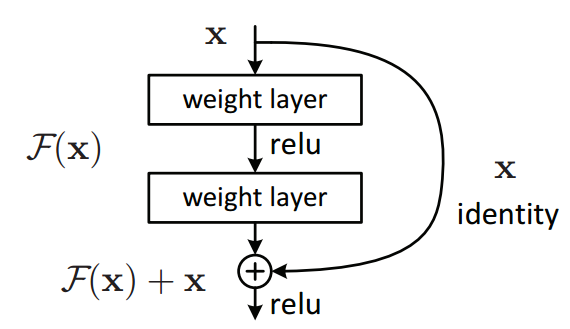
Now, one of the key changes to our CNN model this time is the addition of the residual block, which adds the original input back to the output feature map obtained by passing the input through one or more convolutional layers.
Model Definition:
For ResNet9:
Now if we need to work on a pre-trained model then we will need to make certain changes to it, like changing the number of input and output.
So, for this let us define a function:
Training:
Before we train the model, we will make some small changes:
Now that we are done with the model definition, so let’s evaluate our model before we start the training.
Also, in this technique, we need to set some of the hyperParams too before the training.
After the training, let us visualize the model performance:
Visualization:
We can also plot the lr’s:
So finally, we are done with this model, and come to conclusion that this model is far better than all the previous models. Since in less time it managed to give higher accuracy. If you are interested to see the entire source code: ResNet Code
I have tweaked some of the hyperParams and experimented with the model, You can see in this list:

We can see that within “10min 57s” this model was able to get the accuracy to 67%(approx) which is best till now of all the approaches tried.
You can find the link to the whole Source code for this approach here: ResNet Codes. With this we come to the end of our Facial Expression Recognition Proejct.
Conclusion:
First, we cleaned the dataset, did some pre-processing, and managed to make our own dataset, which is published on Kaggle.
- Dataset: Kaggle Dataset Page
- Kaggle: All Notebooks
- Github Repo: Containing all the codes
Then we tried 4 different approaches to solve our problem:
- Logistic Regression:
—val_loss:1.62971
—val_acc:38%(Approx.)
— Notebook: Link - Feed-Forward Neural Network(FNN):
—val_loss:1.61005
—val_acc:47%(Approx.)
— Notebook: Link - Convolutional Neural Network(CNN):
—val_loss:1.44248
—val_acc:57%(Approx.)
—train_loss:0.61862
— Notebook: Link - CNN with Data Augmentation & Regularization Technique:
—val_loss:0.93374
—val_acc:65%(Approx.)
—train_loss:0.73313
— Notebook: Link
So, in the end we come to the conclusion that CNN with Data Aug. & Reg. Techniques we can attain a good accuracy score, and also if we can figure out some good hyperParams and transformation combinations we may be able to attain an accuracy score of about (70–75)% and deploy our model to even production.
Lastly, I would like to thank Aakash N S Sir for providing us with this course, since the past 6 weeks. I didn’t have any idea about Deep Learning, and today I have successfully managed to build my own model.
If you have made it till here, you can suggest some more techniques or approaches that I should try. If would like to give any feedback, you can connect me on various platforms:
- Kaggle: manishshah120
- LinkedIn: manishshah120
- Twitter: manishshah120
- GitHub: manishshah120
